 |
Research | Summer 1999 |
 |
During the summer of 1999, I worked with
Amy
Bug and Robert
McFarland in the Swarthmore
Physics Department. I am very thankful to have had an opportunity
like this as a rising sophomore undergraduate, for it was a wonderful
learning experience. Our results from that summer are published in "A two-chain path integral model of positronium" in the December 15, 2000 issue of the Journal of Chemical Physics. I spent most of my days in front of our Unix
workstations, Barney and Bert, or our new G3, running programs and
analyzing the output data. I also spent some time finding research papers
in Cornell
Library. I have some pictures of Robert and
I eating lunch.
On July 21, Robert and I gave a presentation about our research to other
students and faculty members who are doing research on campus this summer.
view slideshow
Amy is a computational physicist, and her Fortran 90 program that we
have been working with uses a path integral monte carlo technique to
simulate quantum particles. First, I had to learn Fortran 90. And here
is a little bit of what I have been doing with it:
Anti-Hydrogen
To test Amy's program, we simulated anti-hydrogen, which is similar to
hydrogen but has a positron (positive electron) around a negative nucleus.
This is the wave function from one of these runs. In this run we used 320
beads with beta = 50. The actual anti-hydrogen potential is a Coulomb
potential, but since this goes to negative infinity near the origin, we
used a Yukawa potential with a = 0.1. About 20 beads were moved per
staging pass, and we ran the program for 100,000 passes, subtracting off
the first 10,000 to give the system time to equilibrate before taking
data. The theory for the probability density, drawn with a blue line,
is P(r) = -r * e^(-2r). The black dots represent our data. |
|
 |
Free Positronium
 |
|
Once we found that anti-hydrogen was working, we edited the program to
model positronium. Positronium is formed when an electron and positron
come in contact; it is like the hydrogen atom, with a positron replacing
the proton. The electron and positron quickly annihilate each other; the
singlet state lasts about E-10 seconds, while the triplet state lasts
about E-8 seconds.
This graph demonstrates the theory that as a (the Yukawa
radius) goes to zero and P (the number of beads on each chain representing
a quantum particle) goes to infinity, the model system approaches the
ideal; this theoretically works best if a is kept in proportion to
P^(-2/3). The theoretical 1s curve on this plot is P(r) = r^2 * e^(-r).
This plot was generated after 200,000 staging passes, and with beta=50.
|
Positronium in a Hard Sphere
One of my projects was to change a program Amy made from simulating
anti-hydrogen in a hard sphere to simulating positronium. Here, the
center of mass of the beads was repositioned after each staging pass to be
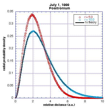
in the center of the cavity. This graph shows the wave function of
positronium in a sphere of radius 5 atomic units and in a sphere of radius
10. Notice that the r=10 curve fits nicely on the 1s theory, while the
smaller sphere forced the electron and positron closer to each other,
making the relative distance between them smaller. This run was done with
P = 320, beta = 50, a = 0.2, and 150,000 staging passes. |
|
 |
 |
|
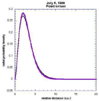
Next I tried unpinning the center of mass. This could become a useful
model for caged positronium, such as in a zeolite cavity. Here is the wave
function of Ps in a sphere of radius 10. The two particles have been
pushed slightly closer together than when their center of mass was pinned,
probably due to when one becomes trapped against the side of the cavity.
This run was done with P = 320, beta = 50, a = 0.2, and 250,000 staging
passes.
Click here for a better picture of Ps in a
cavity, which I used in our slideshow presentation.
|
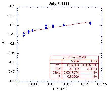
As mentioned before, a Yukawa potential is used to simulate the Coulomb
potential, and our model becomes closer to reality as a goes to zero and P
goes to infinity. Here is my first attempt at extrapolating the energy at
a=0. For each of the 21 runs needed to make this plot, I ran 250,000
staging passes with beta = 50 and the radius of the cavity being 8.0 a.u.
I started with P = 320 and a = 0.2, and I kept the proportion a =
kP^(-2/3) for P = 100, 140, 170, 200, 400, and 600. For each P I did
three statistically independant runs, and it is clear that our energy
estimator is not very precise. Still, with this linear extrapolation we
found an energy of -0.242, which is slightly higher than the ground state
energy of -0.25 due to the hard wall boundary conditions. This P^(-4/3)
scaling was predicted by Muser and Berne, and our plot looks very similar
to theirs on this scale. |
|
 |
 |
|
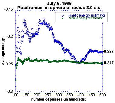
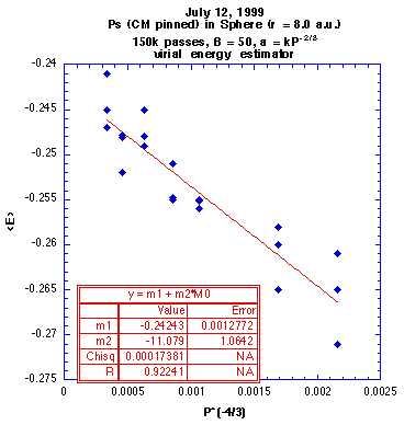
My next project was to examine our energy estimator. Our original
estimator was a kinetic energy estimator, and in an attempt to reduce the
variance I created a new version of our code with a virial energy
estimator. Here is a plot which dramatically demonstrates the steadiness
of the virial estimator compared to the kinetic estimator.
|
Using the virial energy estimator, I did another extrapolation of the
energy in a sphere of radius 8. Again, the best line took us to -0.242,
but with a somewhat better fit (R=0.922 vs. R=0.896).
I tried unpinning the center of mass and doing the same sort of
extrapolation with the virial estimator, and was surprised to find the
energy going below the ground state energy of -0.25. Amy told me that the
virial estimator cannot be used for a particle unpinned in a cavity, since
it does not account for the cavity walls in any way. I used the kinetic
estimator instead, and extrapolated the energy to -0.071 for r=5.0 a.u.
and = -0.189 for r=8.0 a.u. I then added another (small) term into
the energy estimator to better account for the cavity walls, and got some
good results.
|
|
 |
Calculated Energy of Positronium
(using virial energy estimator)
|
Cavity Radius |
Energy |
Potential Energy |
|
Free Ps
10.0 a.u.
8.0 a.u.
6.0 a.u.
5.0 a.u.
4.0 a.u.
|
-0.252 +- 0.004
-0.184 +- 0.006
-0.178 +- 0.005
-0.132 +- 0.004
-0.058 +- 0.005
0.059 +- 0.010
|
-0.500 +- 0.003
-0.522 +- 0.002
(no data)
-0.564 +- 0.003
-0.597 +- 0.002
-0.666 +- 0.002
|
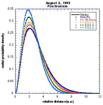
Here is one of my final plots of the radial probability density of
positronium in a hard cavity. As you can see, as the cavity size
decreases and squeezes positronium, the two particles are more likely to
be found close together.
| |
 |