Description:
In this assignment, a graphics library was written to draw points, circles, ellipses and lines. Lines were drawn using Bresenham's line drawing algorithm while circles and ellipses were drawn using a midpoint algorithm. 3D images were drawn using this library in order to demonstrate its capabilities.
Bresenham's Algorithm for lines
Bresenham's line drawing algorithm may be used to produce a close approximation to a true (continuous) line on a screen with finite resolution. This algorithm is one of the earliest algorithms developed in computer graphics. It works by incrementing the x (or y) value from the starting point and keeping track of an error term, the sign of which indicates whether the y (or x) value should be incremented as well.
Rules for the algorithm vary depending on the slope of the line to be drawn. Lines in each of the eight octants have different sets of rules that determine the initial error and whether the y (or x) value should be incremented at each step.
For an in-depth discussion of the algorithm, you can click here for the information Wikipedia's has on it.
For mathematical correctness, the version of the algorithm that was implemented has the coordinate system shifted from the center of the pixel to the bottom left corner, and the line is made to stop one pixel early. The rules for drawing a line of positive slope of less than 1 (a line in the first octant) are:
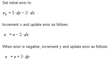
In my implementation, it was ensured that starting points have a lower x-value than ending points. A check for this condition is performed anytime a line is initialized. A line which fails this condition has its starting and ending points swapped. The advantage of this approach is that it cuts the number of octant cases from eight to four. The expressions for drawing lines in the first octant (presented above) may be extended to lines in all other octants by
(a) stepping in y and switching the positions of dx and dy in the error expression when the magnitude of the slope is greater than 1 (i.e in the second and third octants), and
(b) negating dy when slope is negative. Note that it is important to treat vertical and horizontal lines as special cases for the algorithm to work correctly.
After implementing the algorithm, it was tested by drawing lines in all octants as well as horizontal and vertical lines. The resulting image
(see Figure 1) shows that the algorithm works correctly.
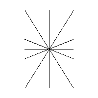
Figure 1. Testing the functionality of the implemented Bresenham's line drawing algorithm
by drawing lines in all octants. The algorithm works as expected.
Midpoint algorithm for circles
The midpoint algorithm may be used to approximate theoretical circles with a finite number of points. The version of the algorithm that was implemented in this assignment calculates points located in one octant only, and reflects these points to all of the remaining octants. The algorithm rules are:
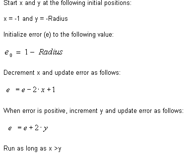
These rules yield a set of points located in the lower half of the third quadrant (i.e. x > y, with x and y both negative). These points must be reflected around the x and y axes to yield points in all of the remaining octants in order to produce a complete circle.
When implementing the algorithm, some guidance was obtained from example code provided by Prof. Bruce Maxwell here.
Midpoint algorithm for ellipses
The algorithm used in drawing ellipses was very similar to that used in drawing circles. It was based largely on example code provided by Prof. Bruce Maxwell (available here). Due to the relative complexity of derivations of the rules for this algorithm, they are not presented in this write-up.
Testing the speed of the Line drawing algorithm :
In order to test the speed of the developed line drawing function, a benchmark program (again, provided by Prof. Bruce Maxwell here) was run on a 2.8 GHz Pentium 4 processor. The image resulting from the test run can be seen in Figure 2 below. Information printed out by the benchmark program indicated that the line drawing function can produce 489,172 lines per second with an average line length of 102.9.
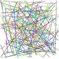
Figure 1. Image produced by the line drawing speed test program. Line drawing program drew 489,173 lines (of average length 102.9) per second.
Required Images:
The first required image was produced using a program provided by Prof. Bruce Maxwell. This image can be seen in Figure 3 below. The image clearly depicts the face of some sort of weird creature. This image portrays that the developed graphics environment ("derelikt.h") can correctly produce lines, ellipses and circles.
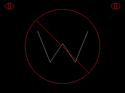
Figure 3. Required image #1: Some sort of weird creature.
The second required image made use of the demonstrated capabilities of the graphics environment to produce a 3D scene. This image can be seen in Figure 4 below. It depicts what can happen to a badly designed camouflaged vehicle on the warfront. The designers forgot to camouflage the tires which resulted in the vehicle being located and assaulted by an enemy flying saucer. Please note that filling in of the elliptical and circular shapes with color in this image was not performed by a fill algorithm, but rather by inefficient repeated drawing of shapes with the same center but varying radii. This was done because at the time of generating the picture, no efficient fill algorithm had been yet developed. It can be observed from the image that the "repeated drawing" fill method does not work very well, as some bits of background color still remain (see sun in Figure 4).
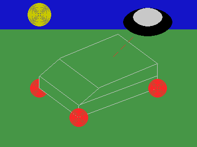
Figure 4. Required image #2: Badly camouflaged military vehicle being assaulted by an enemy flying saucer.
The inefficient fill procedure used to produce the image in Figure 4 was replaced by a seed-fill algorithm as an extension . The seed-fill algorithm is presented in the next section ("Extensions"). For direct comparison, the image produced using the flood algorithm is presented in this section (in Figure 4b below). It is clear that the seed algorithm works much better than the naive method used previously. Notice how background color no longer shows through the car's tires and the sun. It must be mentioned however, that the see-through effect seen in Figure 4 looks cool and may be good for some applications. In particular,
in Figure 4, notice how the effect makes the tires look as if they are spinning.

Figure 4b. Badly camouflaged military vehicle redrawn using a seed-fill algorithm to color in surfaces.
Extensions:
1. The Bouncing Ball
The first extension involved developing the trajectory of a ball which is thrown horizontally at some elevation above ground. Equations of motion (of constant acceleration) were used to determine physically correct location of the ball at different points in time. The different frames were drawn into a single image since at the time of generation, no system had yet been developed to produce GIF animations. Also, the static nature of the image enables its use in the end-of-semester poster session. The ball was made to lose 0.2 of its kinetic energy anytime it collided with the ground. Also, the ball was made to squish into an ellipse anytime it hit the ground. The trajectory is shown in Figure 5.

Figure 5. Trajectory of a ball thrown horizontally at some elevation above ground.
The ball loses 0.2 of its kinetic energy upon contact with ground.
2. Seed fill algorithm and an improved 3D Model
The second extension involved developing a seed-fill algorithm to color in surfaces. My implementation requires as input an image structure, an initial seed point, the boundary color and the fill color. The seed point is placed on a stack, colored and its surrounding four pixels are tested. Surrounding points which are found to not be of the boundary color or the fill color are placed on the stack. Points are taken from the stack, colored, their surrounding points are tested and the process continues until all points within a boundary of specified color are colored appropriately.
The algorithm was then used to develop the 3D model of a spaceship calmly cruising through space. "Curved" portions of the spaceship were created by drawing lines between narrowly separated points. To make this task easier, a function was written to join consecutive entries in an array of points, using the developed line drawing algorithm. This function was included directly in the spaceship drawing program and not in a library for the graphics environment, since a more efficient method (using polygons) is expected to be developed in the next assignment. The finished spaceship model is shown in Figure 6.

Figure 6. What a spaceship looks like in my mind. Surfaces are colored in using a simple seed algorithm.
**Disclaimer: I never claimed to have a vivid imagination.
3. Animating the bouncing ball
Next, it was decided that the bouncing ball image should be made into a .gif animation. In order to make the ball easier to see, its radius was increased. Also, the ball was colored in using the floodfill algorithm. The resulting animation can be seen in Figure 7. Way better looking than the static Figure 5, wouldn't you say?

Figure 7. Bouncing ball .gif animation. The ball is colored in using the floood fill algorithm from Extension #2.
Questions:
Who did you work with on this assignment, and what tasks did each of you do?
This assignment was worked on by Paul alone. However, when Lab 3 was being carried out, it was discovered that the line algorithm had issues with slope values in certain ranges. These problems were solved together with the lab partner at that time, David Wright. As a result, the submitted version of the line algorithm for this assignment is a collaboration between David Wright and Paul Azunre.
Develop an API manual for your graphics environment. This should be a mini-manual on how to use your graphics system. Include the following information in your answer: What state variables do you have and what is their meaning? How do you represent these variables and what are their types? How do users modify/access the state variables? How do the graphics routines access the state variables?
Since most functions that were implemented within the graphics environment are exactly as described by Prof. Bruce Maxwell
in the "Graphics Environment Specifications" (available here), the mini-manual may be summarized as the description of the few additions that were made:
The name of the graphics environment is "derelikt.h". So far, it consists of the following files:
- derelikt.h -- environment header file.
- basic.c -- includes basic functions to initialize primitives.
- line.c -- implements Bresenham's algorithm to draw lines.
- ellipse.c -- implements a midpoint algorithm to draw ellipses.
- circle.c -- implements a midpoint algorithm to draw circles.
In addition to the functions specified in the Graphics Environment Specifications,
the following 2 functions were written to convert between the Color and Pixel types:
- Color *Pix2C(Pixel *pix);
- Pixel *C2Pix(Color *col);
Variables *pix and *col represent pointers to the Color and Pixel types respectively. The functions map the integer color range 0 - 255 (as defined in the Pixel type) into the float color range 0 - 1 (as defined in the Color type) for each color (red, green and blue) and vice versa. They return pointers to the resulting Color or Pixel types as appropriate.
The seed fill algorithm is performed using the following function:
Variables src, start, c and bc represent the image, the initial seed point, the fill color and the boundary color respectively. The function fills an area surrounded by some boundary color (bc) with a color specified as c. For a description of the algorithm see the Extensions section above.
What modifications to the code did you make in order to deal with coordinate system issues such as making lines and circles the proper theoretical size?
In order to make sure that circles and ellipses were of the proper size, reflected values were decremented on a sign change. This was done in order to account for the presence of the origin between the original and reflected values. Lines were made to stop one pixel early in order to not exceed their theoretical length. All of these changes were suggested by Prof. Bruce Maxwell during either class or lab sessions.
If you extended this assignment in any way, describe what you did and how you did it. Include pictures to support your description.
Please see the "Extensions" section above.
|