CS40: Assignment #3: Scan Line Fill Paul Azunre, David Wright
|
||
Description: In this assignment, the scanline fill algorithm was implemented for filling polygons, circles and ellipses with color. Part 1: Scan Line Fill Algorithm for a Polygon General Description The idea behind the scan-line algorithm is to move through the image one line at a time drawing straight lines (filling) between edges of the polygon. The result is a relatively efficient fill (as compared to a flood fill, for instance). Note that while the following algorithm uses horizontal scan lines from bottom to top, this choice is arbitrary. Creating Edge Records
Edges are defined by their start and end points. The first step is to create a record of all the non-horizontal edges. (Horizontal edges don't add to the area filled and should be ignored for this algorithm). Edges are added into an array where the index corresponds to the lower of the two edge points' y values. An upper y-bound is set for the edge equal to the higher of the two edge points' y values - 1 along with the amount x will change per line increment in y (an inverse slope). Once all edges have been added, the actual fill process begins. Line Filling and The Active Edge List
An active edge list is created which holds all the edges which pass through the current (active) scan line. This list is kept sorted by the x-intersect value, that is the edges in the list will be ordered in the active list by where they cross the current scan line from left to right. The algorithm then moves through the active list. If there are edges in it, it checks for the next edge in the list. If there is another edge, the algorithm fills all the pixels on the line between the two edge's x-intersect values. If there is not, it fills until the end of the image line. This process continues until all active edges have been processed. The Next Line
The algorithm then updates the active edge list for the next line. This involves three steps. First, all completed edges (those with upper y-bounds less less than the next line) are removed from the active list. Those remaining have their x-intersect recalculated for the next line (which can be done simply by adding the stored amount x changes per line to the current intersect value). Finally, any edges that begin on the next scan line (those with a lower point y-value equal to the next scan line) are added to the active list and the list is sorted by the updated x-intersect values. The active list for the next line is then processed and the process continues until all scan lines in the image have been finished. Problems With Extrema
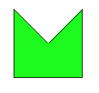
Note that at extrema vertices (polygon vertices which are local y-min or y-max values) the algorithm needs to encounter two edges so that it turns on and then off right away, while at non-extrema vertices the algorithm needs to encounter only a single edge so it will continue to fill (or stop filling, as appropriate). This is achieved by making the upper y-bound in the edge record equal to the upper y point - 1, ensuring that minima vertices will have two edges while others will only have one. But wait, what about maxima vertices? Maxima vertices will be removed from the active list after the scan line immediately before the actual vertex, so they don't need to have two edges at the vertex as the vertex is never reached. Note that this does have some implications for how polygons are defined... namely one should be aware that nothing will be drawn for the line with highest y-value. This actually is somewhat convenient for drawing correct areas as it means the vertical length of the polygon will be correct. A polygon filled with green color using this algorithm may be seen in Figure 1a below.
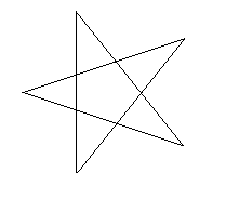
Figure 1a. A polygon filled with color. Other related work included drawing polylines using the previously developed [in lab 2] Bresenham's line drawing algorithm to connect vertices. Figure 1b below shows a polyline drawn in the shape of a Star. Figure 1c shows a filled polygon [the same as in Figure 1a] with a line frame drawn around it. .
Figure 1b. A star-shaped polyline.
Figure 1c. The polygon from Fig 1a with a frame drawn around it. Additionally, clipping was implemented to ensure that polygons with vertices outside of an image could be drawn and that they would maintain their correct shape. An example of a polygon shifted to various positions [at which some of its vertices are outside of an image] can be seen in Figure 1d below.
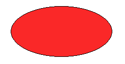
Figure 1d . The polygon shifted to various positions to show that clipping works as expected. . Part 2: Scan Line Fill Algorithm for circles and ellipses For circles and ellipses, the scanline fill algorithm was implemented by modifying previously developed [in lab 2] midpoint algorithms for drawing these primitives. Since the midpoint algorithms already calculate the coordinates of circle and ellipse border pixels, by simply drawing colored horizontal lines between aligned border pixels, the primitive may be completely filled with color. An ellipse and a circles filled with color using this algorithm may be seen in Figures 2b and 2a below.
Figure 2a . A circle filled with color using the scanline algorithm. A frame is drawn around the circle for clarity.
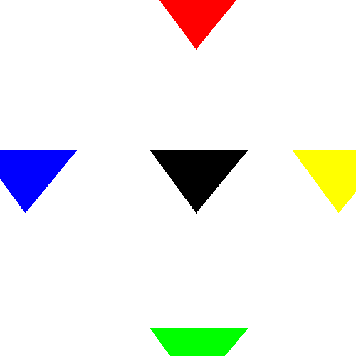
Figure 2b . An ellipse filled with color using the scanline algorithm. A frame is drawn around the ellipse for clarity. Required Images: In order to test the developed scanfill routines, the following image was created using code provided by Prof. Bruce Maxwell.
Figure 3. Required Image #1: A square planet orbiting a tri-colored sun.... Fun stuff.
An image produced for lab 2 was reproduced using scanfill routines to color-in most surfaces. This image can be seen in Figure 4 below.
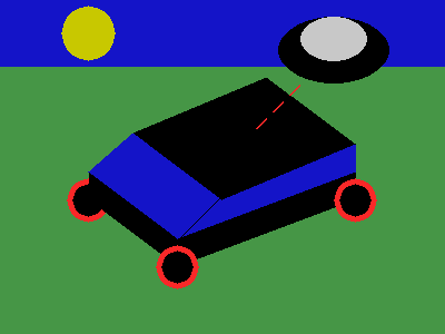
Figure 4. Required Image #2. The previously camouflaged [in lab 2] vehicle decides to blow its cover as it prepares to flee. Questions:
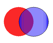
Extensions: Alpha blending: As an extension, alpha blending was attempted for circles and ellipses. For alpha blending, the following expression is used to determine final pixel value:
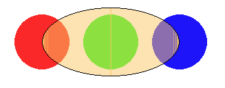
Images of circles and ellipses blended with their background can be seen in Figures 5a and 5b below. Please note that the darker coloring near the edges of alpha blended circles and ellipses is due to some lines being drawn more than once. This bug could not be fixed, but attempts to fix it will be made as the course progresses.
Figure 5a . A circle alpha blended with an opaque circle and a white backround.
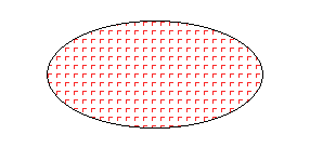
Figure 5b. An ellipse alpha blended with several opaque circles and a white backround. . Pattern Fill: Additionally, a pattern fill was implemented for ellipses. First of all, an 8x8 pixel pattern structure is specified. An anchor point for determining the filled pattern at a pixel within the ellipse is set. For our implementation, the point corresponding to the minimum x-value and y-value of the ellipse is used as the anchor. The final value of a given pixel in the ellipse is then determined based on a modulo 8 operation on the x and y value to map them to a corresponding pixel of the pattern. An example of a very simple (ugly) pattern fill is shown in Figure 6.
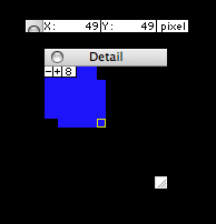
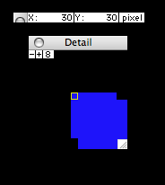
Figure 6. An ellipse with an ugly pattern fill. A simple OpenGL interface: Using the OpenGL skeleton code [provided in lab #2], a simple GUI for a portion of our graphics library was implemented. At present, only a rough framework which can draw filled red circles centered at locations specified by the mouse is functional. The resulting images can be saved to .ppm format via a right-click menu. A screen shot of our GUI in action is shown in Figure 7.
Figure 7 . OpenGl GUI screenshot. Yep, David can be scary sometimes. Animations of the Flood-fill and Scan-line fill Algorithms In order to demonstrate the difference in operation between the scan-line fill algorithm implemented in this lab and the flood-fill algorithm implemented in the previous lab, animations of the algorithms operating on the same shape were generated. These are shown in Figures 8 and 9 below. Note that the lower resolution of the flood-fill animation is due to its very low speed --ridiculous amounts of computational power were required to produce animations of resolution similar to that of the scan-fill animation. In fact, the computer running the code crashed several times while attempting to render at higher resolutions. While this difference makes a direct comparison more difficult, the animations do serve their purpose pretty well. Note that the flood-fill animation takes a much longer time to conclude despite its lower resolution (both images have the same frame rate). This makes it clear that the scan-fill algorithm is a much faster one.
Figure 8. Scan-fill algorithm operation animation.
Figure 9. Flood-fill algorithm operation animation.
Figure 9 also shows one drawback of the four-connected floodfill algorithm. The shape does not fill completely (notice the two white patches at ends of polygon at the conclusion of animation). In this case, an eight-connected algorithm (one that tests all eight pixels surrounding the seed) would work much better. This scenario demonstrates the classic tradeoff -- more computational power/time required vs. greater efficiency.
|
||
© Paul Azunre, 2006 |